ggheatmapper: Tile-able heatmaps that play well with ggplots

Introduction

ggheatmapper is built using ggplot2 and the patchwork framework for aligning plots. It supports adding into the heatmap and all the powerful tweaks enabled by themes in ggplot, and helps you align more information about your data to the original heatmap to make “complex heatmaps” with a more modern and tweakable framework.

Using a matrix as your table

The simplest, yet less powerful, way to use ggheatmapper is with a matrix as-is. Here, we demonstrate with a subset of a gene expression matrix for bladder cancer samples:

library(tidyverse)
#> ── Attaching core tidyverse packages ──────────────────────── tidyverse 2.0.0 ──
#> ✔ dplyr     1.1.3     ✔ readr     2.1.4
#> ✔ forcats   1.0.0     ✔ stringr   1.5.0
#> ✔ ggplot2   3.4.3     ✔ tibble    3.2.1
#> ✔ lubridate 1.9.2     ✔ tidyr     1.3.0
#> ✔ purrr     1.0.2     
#> ── Conflicts ────────────────────────────────────────── tidyverse_conflicts() ──
#> ✖ dplyr::filter() masks stats::filter()
#> ✖ dplyr::lag()    masks stats::lag()
#> ℹ Use the conflicted package (<http://conflicted.r-lib.org/>) to force all conflicts to become errors
library(patchwork)
library(ggheatmapper)
#> Registered S3 methods overwritten by 'treeio':
#>   method              from    
#>   MRCA.phylo          tidytree
#>   MRCA.treedata       tidytree
#>   Nnode.treedata      tidytree
#>   Ntip.treedata       tidytree
#>   ancestor.phylo      tidytree
#>   ancestor.treedata   tidytree
#>   child.phylo         tidytree
#>   child.treedata      tidytree
#>   full_join.phylo     tidytree
#>   full_join.treedata  tidytree
#>   groupClade.phylo    tidytree
#>   groupClade.treedata tidytree
#>   groupOTU.phylo      tidytree
#>   groupOTU.treedata   tidytree
#>   inner_join.phylo    tidytree
#>   inner_join.treedata tidytree
#>   is.rooted.treedata  tidytree
#>   nodeid.phylo        tidytree
#>   nodeid.treedata     tidytree
#>   nodelab.phylo       tidytree
#>   nodelab.treedata    tidytree
#>   offspring.phylo     tidytree
#>   offspring.treedata  tidytree
#>   parent.phylo        tidytree
#>   parent.treedata     tidytree
#>   root.treedata       tidytree
#>   rootnode.phylo      tidytree
#>   sibling.phylo       tidytree

data(tcgaBLCA_ex)
gexp <- tcgaBLCA_ex$gexp

gghm <- ggheatmap(gexp,
          hm_colors = 'RdBu',
          hm_color_values = scales::rescale(c(-4,-2,-1,-0.5,-0.25,0,0.25,0.5,1,2,4,6)),
          scale = TRUE,
          center = TRUE,
          show_dend_row = TRUE,
          colors_title = "Scaled expression (log2 UQ)",
          show_colnames = FALSE)
#> Running `ggheatmap` in matrix mode. If that's not intentional, provide a `colv`.
gghm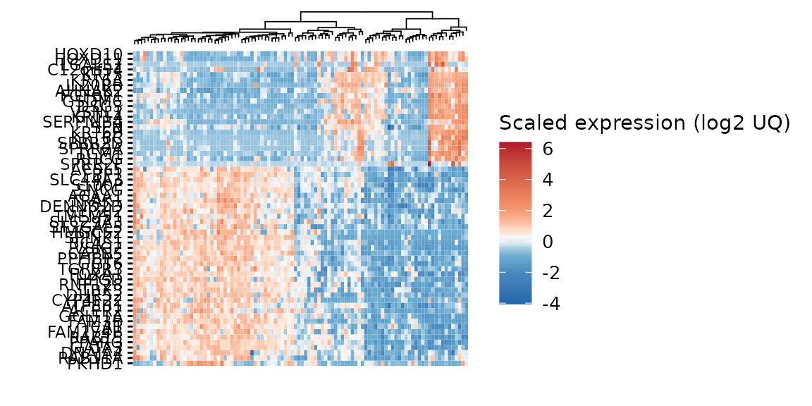

This method still will support extending with align_to_hm but would not support add_tracks. You can still modify this by using & and adding theme, for example:

gghm &
  theme(axis.text = element_text(size = 6))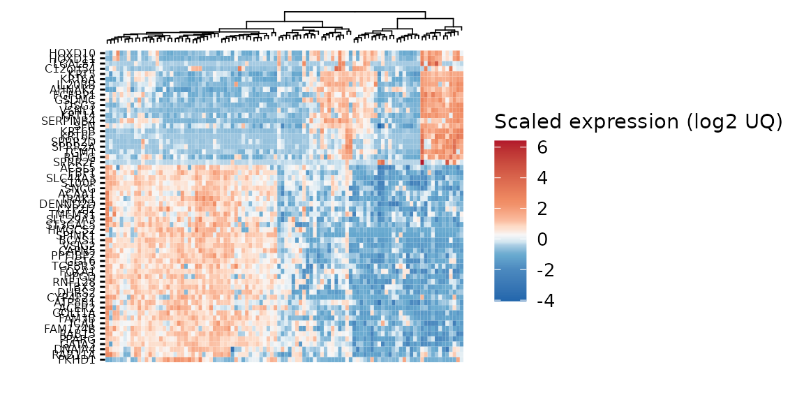

Using tables with more variables

If transpose our original table and extended it with new variables, we can unlock more features using ggheatmap.

sample_annot <- tcgaBLCA_ex$sample_annot %>% as_tibble()
genes <- rownames(gexp)
tcgaBLCA_tb <- gexp %>%
  t() %>%
  as.data.frame() %>%
  rownames_to_column("sample") %>%
  left_join(sample_annot, by = "sample") %>%
  tibble() %>%
  group_by(consensusClass)
head(tcgaBLCA_tb)

sample	FBP1	ACER2	PKHD1	CAPN5	S100P	TMEM51	DHRS2	CYP4F22	SPINK1	ACSL5	ST3GAL5	TBX3	HPGD	TGFBR3	FAM3B	ATP8B1	RNF128	SNCG	SLC44A3	GATA3	PPARG	ICA1	GGT6	RAB11A	TRAK1	VSIG2	BCAS1	RAB15	FAM174B	SLC29A3	FOXA1	GOLT1A	PPFIBP2	DENND2D	ACAA1	DNAJA4	HMGCS2	CYP2J2	VSNL1	KRT14	TGM1	SERPINB4	GSDMC	KRT6A	LGALS7	SFN	SPRR2A	C12orf54	SPRR2D	HOXD11	KRT6C	KRT5	DSG3	KRT6B	HOXD10	IL20RB	RHCG	AHNAK2	SPRR2F	FGFBP1	sex	age	stage	node	metastasis	papillary	squamous	consensusClass	separationLevel	LumP	LumNS	LumU	Stroma.rich	Ba.Sq	NE.like
TCGA-XF-A9SW-01A	3.051428	0.7600492	1.0344884	3.190462	7.252360	4.695958	3.553598	0.0458037	8.070943	5.222600	2.7737241	4.846704	4.195551	5.317267	3.1750867	4.278225	3.175087	4.8426545	2.011588	5.840220	4.209453	2.770317	3.728798	5.853159	4.839407	3.2770249	0.9406215	4.783051	3.517479	3.205675	2.9853829	3.279423	2.467868	3.198088	3.772022	3.682428	0.3495844	0.718229	0.6896599	0.8271634	0.5215371	0.0230836	1.3219281	0.2937312	0.0000000	6.262246	1.2842084	0.3856537	0.2552571	0.1118929	0.0230836	1.853159	0.0000000	0.0000000	0.3677318	0.5052353	1.8786937	5.6623525	0.0000000	0.0901978	M	85	T3	N2	NA	0	0	Stroma-rich	0.8871657	0.3931646	0.4925222	0.4609638	0.6421217	0.4954034	0.2989414
TCGA-BL-A13J-01B	2.538652	4.4439186	0.2504068	2.982211	4.283709	2.692439	8.245226	1.7312968	3.901222	4.771899	3.2720427	5.745076	5.665011	4.000000	1.6374299	5.595922	5.496664	1.4043903	3.260282	5.052941	5.196140	3.543512	2.441317	5.449971	5.443269	3.0979633	1.8087013	3.592799	3.937369	1.390071	2.4585741	1.371969	3.780845	3.206136	3.224412	6.407171	2.1814040	2.950846	0.0554951	3.5974805	0.9714308	0.4360991	0.6614754	2.7732793	0.0000000	3.995869	1.0093987	0.0187366	0.7026141	0.5499671	0.0372329	4.684393	1.3756074	0.2264279	1.1477536	0.9952776	2.3462385	4.5877101	0.0093987	0.6909794	M	65	T4	N2	M0	1	0	LumP	0.8960881	0.5418487	0.4977683	0.5031495	0.4995555	0.4950211	0.1822938
TCGA-C4-A0F1-01A	1.532221	2.0437214	3.0887679	2.473487	4.091374	3.335184	4.318595	0.2255597	1.804181	1.606989	0.8845228	2.225560	1.054448	1.599684	0.1475572	4.381709	3.059781	0.9888594	2.791413	4.214842	1.739183	2.461448	1.022026	6.647846	5.364572	0.1273793	0.2255597	1.562595	1.524527	2.191951	0.2630344	0.000000	2.592342	3.752419	4.852614	5.689729	0.0000000	2.566347	5.9933957	14.1342548	1.5700892	8.6758485	4.1235643	13.8688908	0.3526716	10.493024	4.8144715	0.5923420	5.0302002	3.5341382	10.4124884	13.898507	10.7761166	11.8531476	4.1056265	8.1470875	6.8639003	10.1725237	0.4533656	6.4604401	M	71	T3	N0	M0	0	1	Ba/Sq	0.8163011	0.2997577	0.2315946	0.2387890	0.3410051	0.6597589	0.1615142
TCGA-BT-A20W-01A	5.978460	5.0488941	1.2202661	4.915787	7.032628	4.972314	8.033026	5.0979235	8.851008	6.831062	5.1470213	7.443114	6.536437	4.238503	4.1879897	5.445847	5.888681	8.1717314	4.009266	7.773360	6.569229	4.644451	6.227231	6.769685	6.237912	5.8543865	5.1486993	5.892191	3.999070	4.605880	5.4792386	2.973734	5.580307	4.923159	5.437634	5.724268	6.6118234	2.794550	0.1280076	2.5370783	0.9314686	0.0000000	0.2949049	0.9157870	0.0000000	5.650089	0.0294438	0.1143327	0.1143327	0.5599585	0.0147970	2.134797	0.0725125	0.0865877	0.8009666	0.7399372	0.4335102	1.3009540	0.0000000	0.1814469	M	71	T2	N0	M0	0	0	LumU	0.0257908	0.7403699	0.7359217	0.7420607	0.6170841	0.4691149	0.2982330
TCGA-GV-A40G-01A	6.027991	3.9534802	2.8433655	7.060945	6.679805	5.813682	4.730013	5.1503722	9.804690	3.986061	3.8487674	7.189749	6.635844	4.667193	4.3252536	5.299278	6.732415	8.4981895	3.684128	5.840269	5.940347	4.537487	5.706403	7.319151	6.190736	5.8231222	5.0257784	6.155207	4.876234	4.512908	4.8017954	2.762267	5.332157	4.636290	5.964363	5.688439	5.1330829	2.457413	0.1171835	2.3351842	1.6322682	0.3699496	0.2444187	0.2160369	0.0110552	6.640857	0.1674567	0.1475572	0.0756643	0.7458165	0.0220263	2.471488	0.0000000	0.0756643	1.1968007	0.6849913	1.3996970	0.1968007	0.0000000	0.7785321	M	77	T2	N0	NA	0	0	LumU	0.0748451	0.6734381	0.6157098	0.6832107	0.4895690	0.4171794	0.2647129
TCGA-HQ-A2OE-01A	5.562190	5.3558523	3.5948780	5.413716	7.054534	5.541404	6.580083	1.1238717	7.464341	6.386977	5.2531547	9.160480	8.112341	5.058496	6.3492774	7.093522	5.697183	7.7692337	4.639871	7.434341	6.044997	3.523129	4.547161	7.047030	6.513904	4.4078684	5.1383513	6.474951	4.267174	4.653376	7.2894147	5.716423	6.040620	5.575813	5.173789	5.508778	9.2317177	7.126793	0.0099155	0.6842771	0.7449034	0.0774788	0.3436529	0.5682838	0.0000000	8.060994	0.0962153	0.2037952	0.9338331	0.0099155	0.0099155	4.418143	0.6529809	0.1599409	0.2630344	0.5548005	1.1820347	0.3975197	0.0000000	0.1329739	M	69	T2	N2	NA	1	0	LumP	0.3120613	0.6270255	0.5555841	0.5852272	0.4305816	0.4076061	0.2394613

One of the additional features we unlock is using grouping with group_by to make semi-supervised heatmaps. In this case, we need to say which column contains the IDs that will be the columns of the heatmap (in this case, colv = 'sample'), and what are the columns we want to plot as rows (rowv = genes). Other parameters here are graphical, for demonstration:

gr_gghm <- ggheatmap(tcgaBLCA_tb,
    colv = "sample",
    rowv = genes,
    hm_colors = 'RdBu',
    hm_color_values = scales::rescale(c(-4,-2,-1,-0.5,-0.25,0,0.25,0.5,1,2,4,6)),
    scale = TRUE,
    center = TRUE,
    show_dend_row = FALSE,
    show_colnames = FALSE,
    show_rownames = FALSE,
    group_colors = c(`Ba/Sq` = "#fe4a49", LumNS = "#32837d", LumP = "#06d6a0", LumU = "#009fb7",
                     `Stroma-rich` = "#f9c80e", `NE-like` = "#7d5ba6"),
    colors_title = "Scaled expression (log2 UQ)")

gr_gghm +
  plot_layout(guides = 'collect')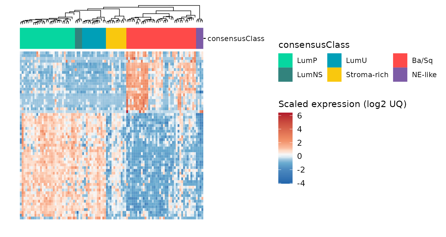

Here, we can see that the heatmap is clustered in a semi-supervised manner (by consensusClass). It also enables add_tracks:

Adding tracks

You can add_tracks for variables that were in the original table fed to ggheatmap. You can see what variables are available using get_data:

get_data(gr_gghm) %>% colnames()
#>  [1] "observations"    "FBP1"            "ACER2"           "PKHD1"          
#>  [5] "CAPN5"           "S100P"           "TMEM51"          "DHRS2"          
#>  [9] "CYP4F22"         "SPINK1"          "ACSL5"           "ST3GAL5"        
#> [13] "TBX3"            "HPGD"            "TGFBR3"          "FAM3B"          
#> [17] "ATP8B1"          "RNF128"          "SNCG"            "SLC44A3"        
#> [21] "GATA3"           "PPARG"           "ICA1"            "GGT6"           
#> [25] "RAB11A"          "TRAK1"           "VSIG2"           "BCAS1"          
#> [29] "RAB15"           "FAM174B"         "SLC29A3"         "FOXA1"          
#> [33] "GOLT1A"          "PPFIBP2"         "DENND2D"         "ACAA1"          
#> [37] "DNAJA4"          "HMGCS2"          "CYP2J2"          "VSNL1"          
#> [41] "KRT14"           "TGM1"            "SERPINB4"        "GSDMC"          
#> [45] "KRT6A"           "LGALS7"          "SFN"             "SPRR2A"         
#> [49] "C12orf54"        "SPRR2D"          "HOXD11"          "KRT6C"          
#> [53] "KRT5"            "DSG3"            "KRT6B"           "HOXD10"         
#> [57] "IL20RB"          "RHCG"            "AHNAK2"          "SPRR2F"         
#> [61] "FGFBP1"          "sex"             "age"             "stage"          
#> [65] "node"            "metastasis"      "papillary"       "squamous"       
#> [69] "neuroendocrine"  "plasmacytoid"    "consensusClass"  "cor_pval"       
#> [73] "separationLevel" "LumP"            "LumNS"           "LumU"           
#> [77] "Stroma.rich"     "Ba.Sq"           "NE.like"

observations will always be your ID variable, which is a factor ordered in the same way as the heatmap, to ease making new plots that will be perfectly aligned. Here, we’ll add some clinical tracks:

gr_gghm <- add_tracks(gr_gghm,
           track_columns = c("stage", "node", "metastasis"),
           track_colors = list(stage = 'Greys', node = 'Oranges', metastasis = 'Reds'),
           track_prop = 0.2)
#> Adding missing grouping variables: `consensusClass`
gr_gghm +
  plot_layout(guides = 'collect')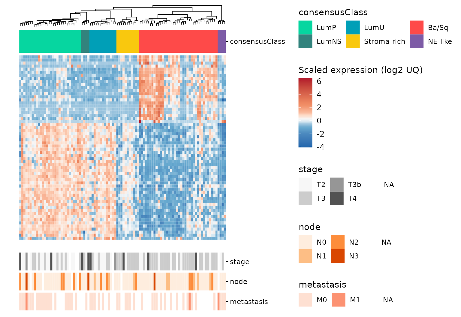

Aligning new plots

Here we’ll make two different plots: one to align with the samples (columns) and another to align with the genes (rows). We can get the data from get_data, which is a good idea to facilitate further plotting because it will ensure your observations will be in the correct order. Then, here, we make a line-plot with the correlations of each sample to the centroid of the 6 consensus bladder cancer subtypes. Note the use of theme_quant, one of our suggested themes that look nice with ggheatmaps, and that we switch the y-axis to the right side to make the end-product look better (though everything will work without this):

tcgaBLCA_tb2 <- get_data(gr_gghm)
plt_corlines <- tcgaBLCA_tb2 %>%
  ungroup() %>%
  select(observations, LumP:NE.like) %>%
  pivot_longer(cols = -observations, names_to = "subtype", values_to = "cor") %>%
  ggplot(aes(observations, cor, color = subtype, group = subtype)) +
  geom_line() +
  scale_y_continuous(position = "right") +
  scale_color_manual(values = c(`Ba.Sq` = "#fe4a49", LumNS = "#32837d", LumP = "#06d6a0", LumU = "#009fb7",
                                `Stroma.rich` = "#f9c80e", `NE.like` = "#7d5ba6")) +
  guides(color = FALSE) +
  labs(y = "Correlation\n to centroid") +
  theme_quant()
#> Warning: The `<scale>` argument of `guides()` cannot be `FALSE`. Use "none" instead as
#> of ggplot2 3.3.4.
#> This warning is displayed once every 8 hours.
#> Call `lifecycle::last_lifecycle_warnings()` to see where this warning was
#> generated.
plt_corlines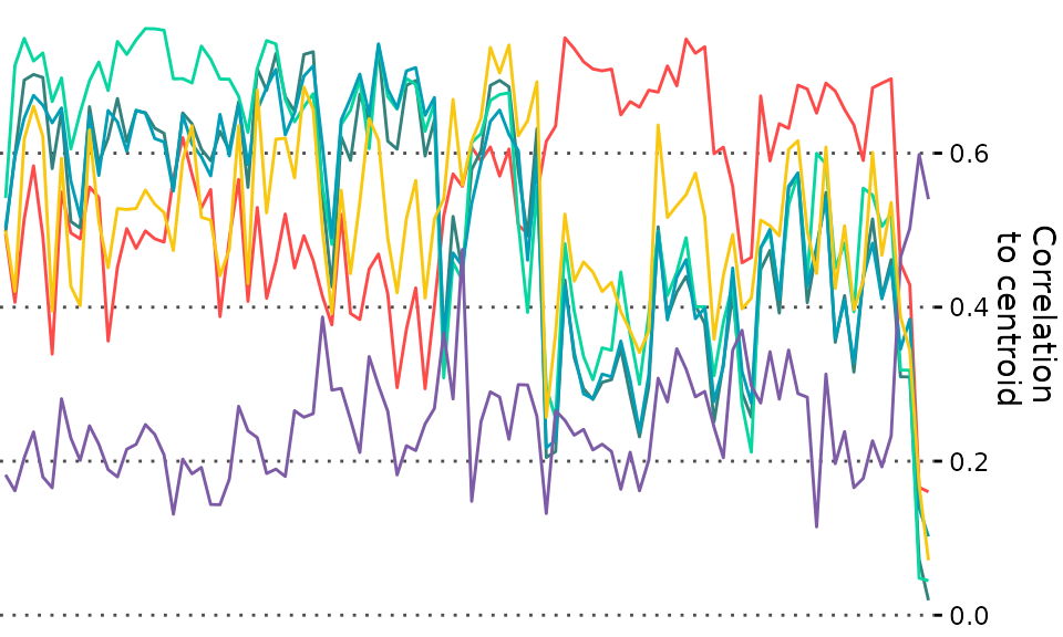

The second plot should align to the rows. We can’t just use the get_data because it doesn’t contain the information to order our rows, but we can get this from get_rowLevels. Here, we plot which signature each gene in our example data belongs to:

plt_row_annot <- tcgaBLCA_ex$gene_annot %>%
  mutate(gene_symbol = factor(gene_symbol, levels = get_rowLevels(gr_gghm)),
         group = 'signature') %>%
  ggplot(aes(gene_symbol, group, fill = signature)) +
  geom_tile() +
  labs(y = "") +
  coord_flip() +
  theme_sparse2()
plt_row_annot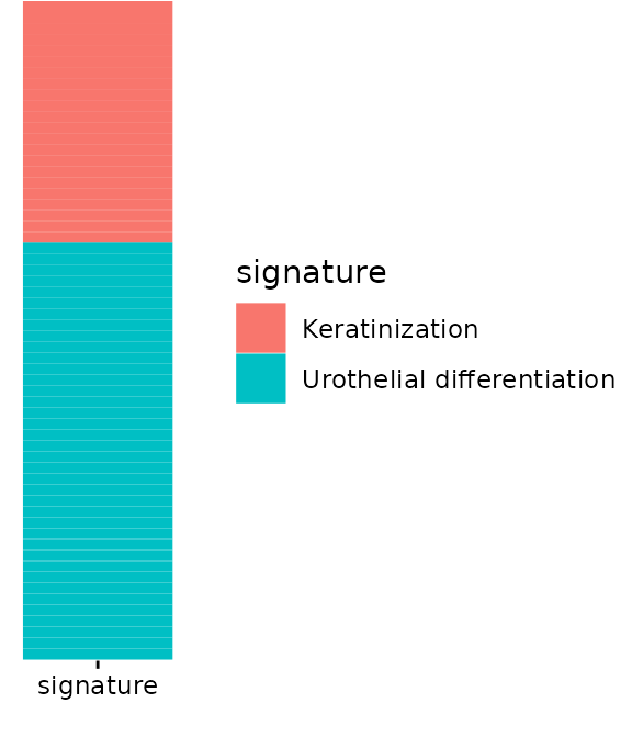

Finally, we can use align_to_hm to add these plots to the original hm with all panels properly aligned. Note the use of legend_action = 'collect' in the final call, that will unite all the legends in a nice way:

gghm_complete <- gr_gghm %>%
  align_to_hm(plt_corlines, newplt_size_prop = 0.3) %>%
  align_to_hm(plt_row_annot, pos = "left", newplt_size_prop = 0.08, 
              legend_action = "collect", tag_level = 'keep')
gghm_complete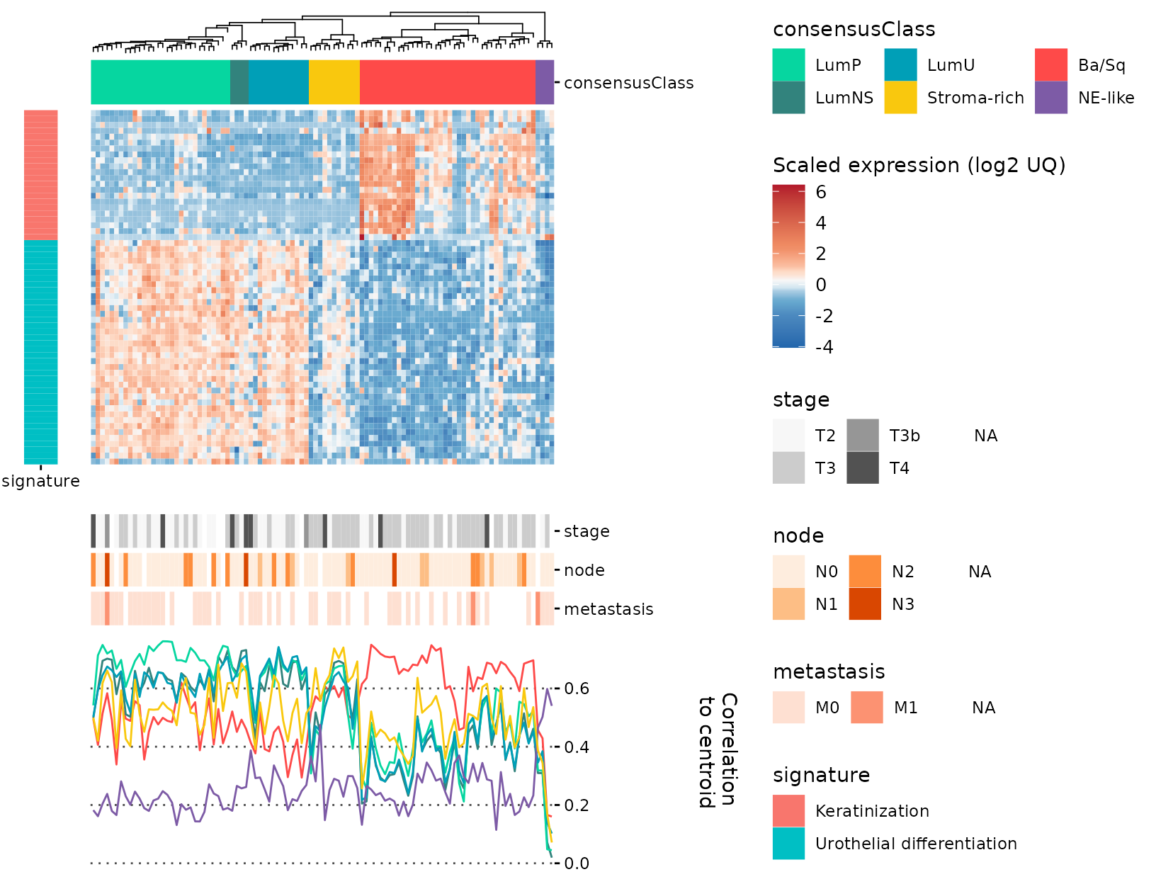

Note that you can still use the patchwork & to make global changes to all plots:

gghm_complete <- gghm_complete &
  theme(legend.text = element_text(size = 7),
        legend.title = element_text(size = 8))
gghm_complete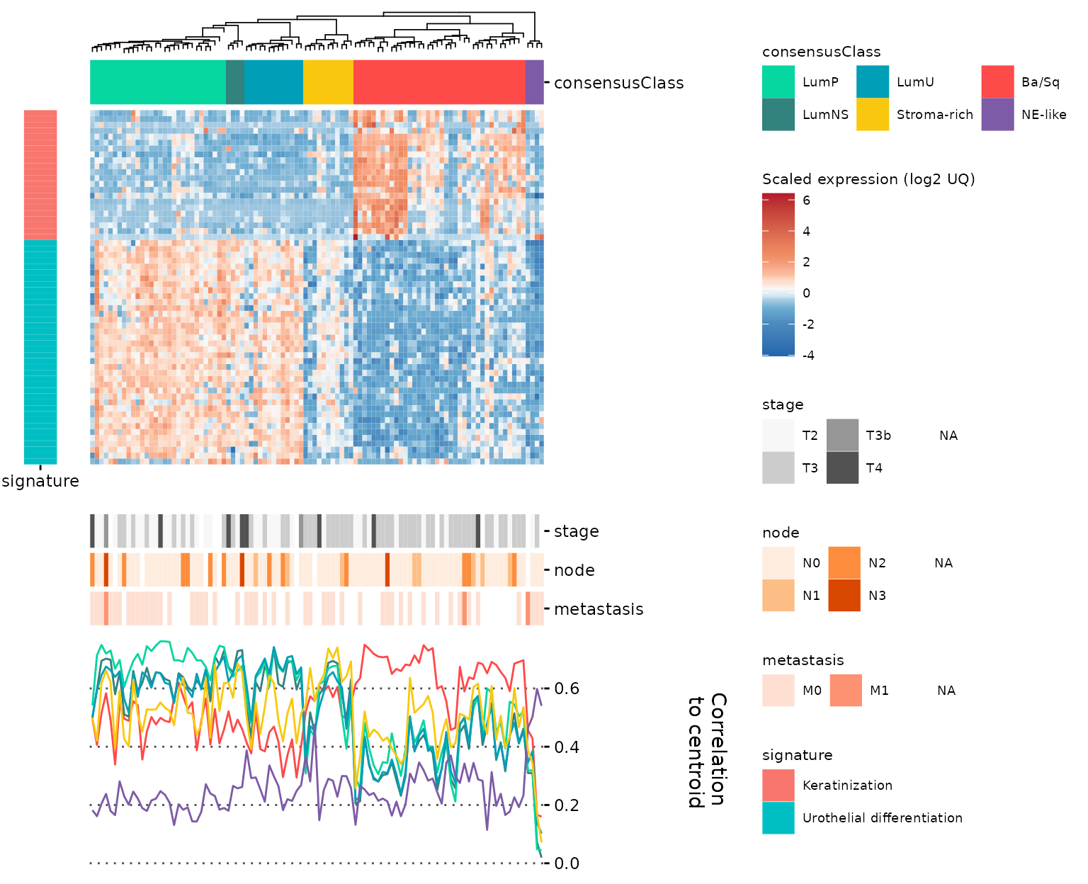

Creating panels

You can now make panels with your complete heatmap with patchwork, cowplot or other aligning packages. For example:

plt_subtype_count <- ggplot(sample_annot, aes(consensusClass, fill = consensusClass)) +
  geom_bar() +
  scale_fill_manual(values = c(`Ba/Sq` = "#fe4a49", LumNS = "#32837d", 
                               LumP = "#06d6a0", LumU = "#009fb7",
                                `Stroma-rich` = "#f9c80e", 
                               `NE-like` = "#7d5ba6")) +
  labs(y = 'Number of samples') +
  guides(fill = FALSE) +
  theme_quant() +
  theme(axis.ticks.x = element_line(color = "black"),
        axis.text.x = element_text(color = "black", angle = 45, hjust = 1, vjust = 1))

plt_subtype_count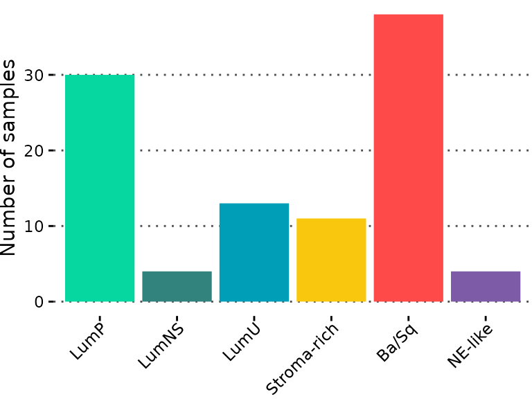

Then, we can just use standard patchwork to align the ggheatmap and our new plots (as they won’t be aligned with the heatmap part of the plot, but with the entire plot):

library(patchwork)
new_col <- (plt_subtype_count + plot_spacer()) +
  plot_layout(heights = c(0.3,0.7))

(new_col | gghm_complete) +
  plot_layout(widths = c(0.4,0.6))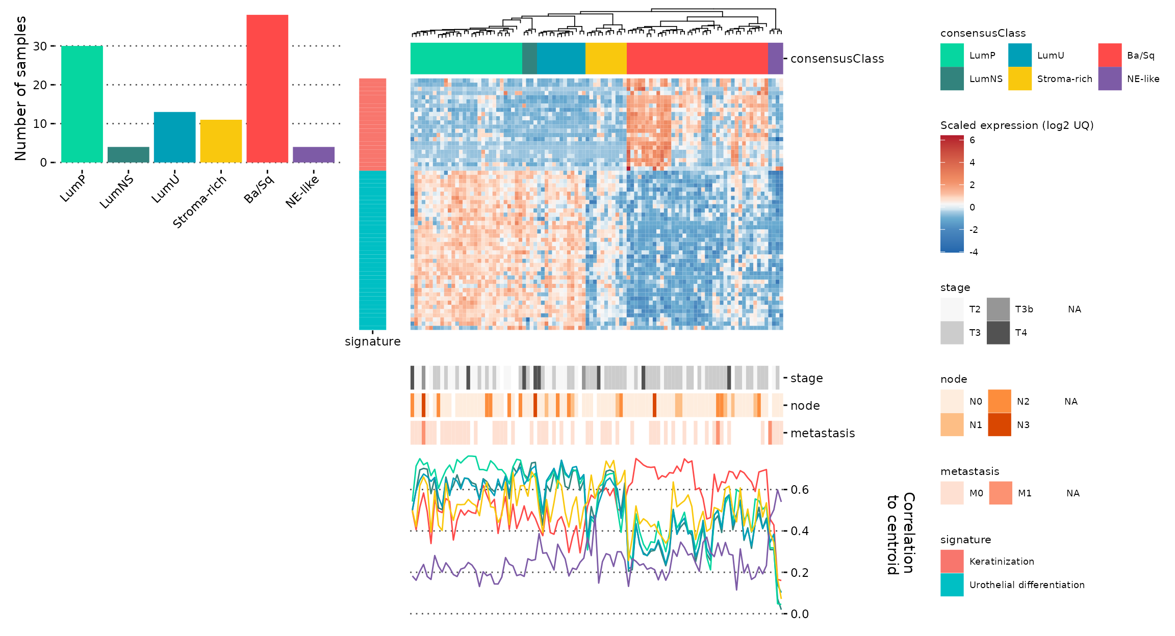

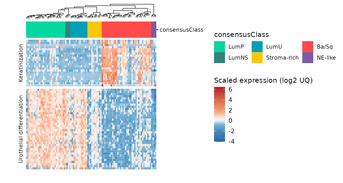
Row facetting

As of ggheatmapper 0.1.2, we’ve added row facetting options using the rowv parameter. ggheatmapper will render parts of the heatmap in different facets if the rowv argument for the ggheatmap call is a named list:

sig_list <- split(tcgaBLCA_ex$gene_annot$gene_symbol, tcgaBLCA_ex$gene_annot$signature)

gr_gghm <- ggheatmap(tcgaBLCA_tb,
    colv = "sample",
    rowv = sig_list,
    hm_colors = 'RdBu',
    hm_color_values = scales::rescale(c(-4,-2,-1,-0.5,-0.25,0,0.25,0.5,1,2,4,6)),
    scale = TRUE,
    center = TRUE,
    show_dend_row = FALSE,
    show_colnames = FALSE,
    show_rownames = FALSE,
    group_colors = c(`Ba/Sq` = "#fe4a49", LumNS = "#32837d", LumP = "#06d6a0", LumU = "#009fb7",
                     `Stroma-rich` = "#f9c80e", `NE-like` = "#7d5ba6"),
    colors_title = "Scaled expression (log2 UQ)")

gr_gghm +
  plot_layout(guides = 'collect')

Clarice S. Groeneveld